Logistic Regression from Scratch

In this blog, we will describe Logistic Regression from Scratch.

Basically, Logistic regression, a fundamental machine learning algorithm, serves as the cornerstone for binary classification tasks, spam email detection, and so much more. As a matter of fact, implementing logistic regression from scratch for binary classification involves several steps, including defining the logistic function, implementing gradient descent for optimization, and visualizing the results.

Logistic Regression from Scratch: Binary Classification

The following section shows a step-by-step explanation of the different concepts in the provided program for logistic regression.

Import Necessary Libraries:

import numpy as np
import matplotlib.pyplot as plt
from sklearn.metrics import roc_curve, auc

At first, we import the required libraries: NumPy for numerical operations, Matplotlib for plotting, and Scikit-Learn for calculating the ROC curve.

Generate Synthetic Data

np.random.seed(0)
num_samples = 100
X = np.random.randn(num_samples, 2)
y = (X[:, 0] + X[:, 1] > 0).astype(int)

In this example, we generate synthetic data with two features (X) and a binary target variable (y). Further, the target variable is created based on a simple rule: if the sum of the two features is greater than zero, the target is set to 1. Otherwise, it’s set to 0.

Define the Logistic Function (Sigmoid)

def sigmoid(z):
    return 1 / (1 + np.exp(-z))

Then, we define the logistic (sigmoid) function, which maps any input to the range [0, 1]. Basically, this function is used to model the probability of an example belonging to class 1.

Initialize Model Parameters

theta = np.zeros(3)  # Including a bias term

Next, we initialize the model parameters, including a bias term. In this case, there are three parameters (bias, feature 1 coefficient, and feature 2 coefficient).

Add a Bias Term

X_bias = np.column_stack((np.ones(num_samples), X))

We add a bias term (a column of ones) to the input features. Actually, this is a common practice in logistic regression.

Define Hyperparameters

learning_rate = 0.01
num_iterations = 10000

After that, we define hyperparameters for the optimization process, such as the learning rate and the number of iterations for gradient descent.

Gradient Descent for Logistic Regression

for i in range(num_iterations):
    logits = np.dot(X_bias, theta)
    y_pred = sigmoid(logits)
    gradient = np.dot(X_bias.T, (y_pred - y)) / num_samples
    theta -= learning_rate * gradient

Further, we implement gradient descent to optimize the logistic regression model’s parameters. In each iteration, we calculate the logits (linear combination of features and parameters), predicted probabilities, and the gradient of the cost function with respect to the parameters. Then, we then update the parameters using gradient descent.

Plot the Decision Boundary

x_min, x_max = X[:, 0].min() - 1, X[:, 0].max() + 1
y_min, y_max = X[:, 1].min() - 1, X[:, 1].max() + 1
xx, yy = np.meshgrid(np.arange(x_min, x_max, 0.01), np.arange(y_min, y_max, 0.01))
Z = sigmoid(np.dot(np.column_stack((np.ones(xx.ravel().shape), xx.ravel(), yy.ravel())), theta))
Z = Z.reshape(xx.shape)

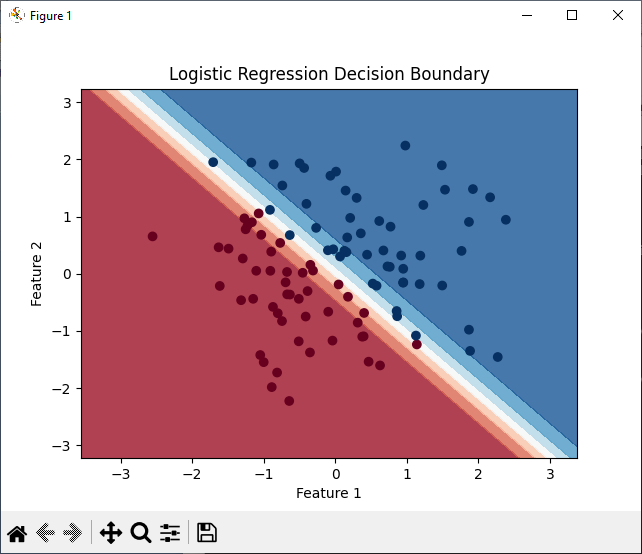
We create a mesh grid to generate a decision boundary. The decision boundary separates the two classes based on the logistic regression model’s predictions.

Plot the ROC Curve

fpr, tpr, _ = roc_curve(y, y_pred)
roc_auc = auc(fpr, tpr)

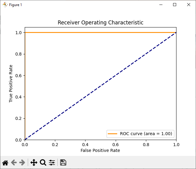
We calculate the Receiver Operating Characteristic (ROC) curve and the area under the curve (AUC) to evaluate the model’s performance.

Plot the Results

plt.contourf(xx, yy, Z, cmap=plt.cm.RdBu, alpha=0.8)
plt.scatter(X[:, 0], X[:, 1], c=y, cmap=plt.cm.RdBu)
plt.xlabel('Feature 1')
plt.ylabel('Feature 2')
plt.title('Logistic Regression Decision Boundary')
plt.show()

Finally, we plot the decision boundary along with the synthetic data points to visualize the classification.

plt.figure()
plt.plot(fpr, tpr, color='darkorange', lw=2, label=f'ROC curve (area = {roc_auc:.2f})')
plt.plot([0, 1], [0, 1], color='navy', lw=2, linestyle='--')
plt.xlim([0.0, 1.0])
plt.ylim([0.0, 1.05])
plt.xlabel('False Positive Rate')
plt.ylabel('True Positive Rate')
plt.title('Receiver Operating Characteristic')
plt.legend(loc='lower right')
plt.show()

Also, we plot the ROC curve to visualize the model’s ability to distinguish between the two classes.

Complete Program

The following code shows the complete Python program that demonstrates these steps using synthetic data.

import numpy as np
import matplotlib.pyplot as plt
from sklearn.metrics import roc_curve, auc

# Generate synthetic data with two classes
np.random.seed(0)
num_samples = 100
X = np.random.randn(num_samples, 2)
y = (X[:, 0] + X[:, 1] > 0).astype(int)  # Create a binary classification problem

# Define the logistic function
def sigmoid(z):
    return 1 / (1 + np.exp(-z))

# Initialize model parameters
theta = np.zeros(3)  # Including a bias term

# Add a bias term to the input features
X_bias = np.column_stack((np.ones(num_samples), X))

# Define hyperparameters
learning_rate = 0.01
num_iterations = 10000

# Implement gradient descent for logistic regression
for i in range(num_iterations):
    # Calculate the logits
    logits = np.dot(X_bias, theta)
    
    # Calculate predicted probabilities
    y_pred = sigmoid(logits)
    
    # Calculate the gradient of the cost function
    gradient = np.dot(X_bias.T, (y_pred - y)) / num_samples
    
    # Update model parameters using gradient descent
    theta -= learning_rate * gradient

# Plot the decision boundary
x_min, x_max = X[:, 0].min() - 1, X[:, 0].max() + 1
y_min, y_max = X[:, 1].min() - 1, X[:, 1].max() + 1
xx, yy = np.meshgrid(np.arange(x_min, x_max, 0.01), np.arange(y_min, y_max, 0.01))
Z = sigmoid(np.dot(np.column_stack((np.ones(xx.ravel().shape), xx.ravel(), yy.ravel())), theta))
Z = Z.reshape(xx.shape)

plt.contourf(xx, yy, Z, cmap=plt.cm.RdBu, alpha=0.8)
plt.scatter(X[:, 0], X[:, 1], c=y, cmap=plt.cm.RdBu)
plt.xlabel('Feature 1')
plt.ylabel('Feature 2')
plt.title('Logistic Regression Decision Boundary')
plt.show()

# Calculate ROC curve
fpr, tpr, _ = roc_curve(y, y_pred)
roc_auc = auc(fpr, tpr)

# Plot ROC curve
plt.figure()
plt.plot(fpr, tpr, color='darkorange', lw=2, label=f'ROC curve (area = {roc_auc:.2f})')
plt.plot([0, 1], [0, 1], color='navy', lw=2, linestyle='--')
plt.xlim([0.0, 1.0])
plt.ylim([0.0, 1.05])
plt.xlabel('False Positive Rate')
plt.ylabel('True Positive Rate')
plt.title('Receiver Operating Characteristic')
plt.legend(loc='lower right')
plt.show()

Output

To summarize, implementing logistic regression from scratch involves the following.

1. To begin with, we generate synthetic data with two classes (0 and 1) using NumPy.
2. Then, we define the logistic function (sigmoid function) to model the probability of belonging to class 1.
3. After that, we initialize the model parameters (including a bias term) and define hyperparameters such as the learning rate and the number of iterations.
4. Then, we implement gradient descent to optimize the logistic regression model’s parameters.
5. In order to visualize the classification, we plot the decision boundary.
6. Finally, we calculate and plot the Receiver Operating Characteristic (ROC) curve to evaluate the model’s performance.

---

Further Reading

How to Perform Dataset Preprocessing in Python?

Spring Framework Practice Problems and Their Solutions

How to Implement Linear Regression from Scratch?

Java Practice Exercise

How to Implement Gradient Descent Algorithm for Linear Regression?

Getting Started with Data Analysis in Python

The Benefits of Using Data Science in the Mortgage Industry: Better Outcomes for Borrowers and Lenders

Wake Up to Better Performance with Hibernate

Data Science in Insurance: Better Decisions, Better Outcomes

Most Popular Trading Software

Breaking the Mold: Innovative Ways for College Students to Improve Software Development Skills

• Angular
• ASP.NET
• C
• C#
• C++
• CSS
• Dot Net Framework
• HTML
• IoT
• Java
• JavaScript
• Kotlin
• PHP
• Power Bi
• Python
• Scratch 3.0
• TypeScript
• VB.NET

Princites