How to Implement Gradient Descent Algorithm for Linear Regression?

The following program demonstrates How to Implement Gradient Descent Algorithm for Linear Regression.

Problem Statement

Implement the gradient descent algorithm for linear regression with one variable from scratch in vectorize form. Train a linear regression model using gradient descent to find the optimal coefficients (slope and intercept) for a given dataset. Also Plot the Gradient Descent.

Solution

The following code shows an implementation of the gradient descent algorithm for linear regression with one variable in vectorized form. Also, we’ll train a linear regression model using gradient descent and plot the progress of gradient descent.

import numpy as np
import matplotlib.pyplot as plt

# Generate sample data
np.random.seed(0)
X = 2 * np.random.rand(100, 1)
Y = 4 + 3 * X + np.random.rand(100, 1)

# Add a column of ones to X for the intercept term
X_b = np.c_[np.ones((100, 1)), X]

# Define hyperparameters
learning_rate = 0.01
num_iterations = 1000

# Initialize the coefficients (theta) randomly
theta = np.random.randn(2, 1)

# Lists to store the history of cost and theta values
cost_history = []

# Gradient Descent
for iteration in range(num_iterations):
    # Calculate predictions using current theta
    predictions = X_b.dot(theta)
    
    # Calculate the errors
    errors = predictions - Y
    
    # Calculate the gradient vector
    gradient = 2 * X_b.T.dot(errors) / len(X_b)
    
    # Update theta using the gradient and learning rate
    theta = theta - learning_rate * gradient
    
    # Calculate the cost (mean squared error) and store it in the history
    cost = np.mean(errors**2)
    cost_history.append(cost)

# Extract the final values of theta (slope and intercept)
intercept, slope = theta

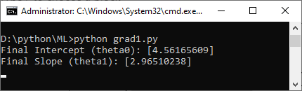
# Print the final coefficients
print("Final Intercept (theta0):", intercept)
print("Final Slope (theta1):", slope)

# Predict Y for the entire dataset
predicted_Y = X_b.dot(theta)

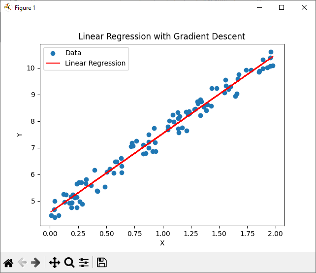
# Plot the original data points and the linear regression line
plt.scatter(X, Y, label='Data')
plt.plot(X, predicted_Y, color='red', label='Linear Regression')
plt.xlabel('X')
plt.ylabel('Y')
plt.title('Linear Regression with Gradient Descent')
plt.legend()

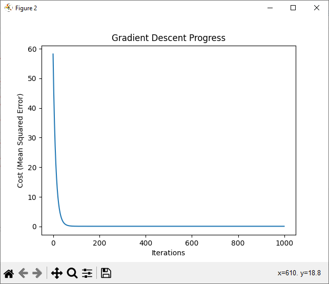
# Plot the gradient descent progress (cost vs. iterations)
plt.figure()
plt.plot(range(num_iterations), cost_history)
plt.xlabel('Iterations')
plt.ylabel('Cost (Mean Squared Error)')
plt.title('Gradient Descent Progress')
plt.show()

Output

In this code:

At first, we generate some sample data (X and Y) to work with.
After that, we add a column of ones to X to account for the intercept term.
Then, we initialize the coefficients (theta) randomly.
After that, we use vectorized operations to perform gradient descent, which makes the code more efficient.
The cost (mean squared error) is calculated and stored at each iteration for later plotting.
After running gradient descent, we extract the final coefficients (intercept and slope).
Further, we plot the original data points and the linear regression line.
Finally, we also plot the progress of gradient descent by showing how the cost changes with each iteration.

Furthermore, you can replace the sample data with your own dataset to perform linear regression on real-world data.

How to Implement Gradient Descent Algorithm for Linear Regression?

Problem Statement

Solution

Further Reading

Leave a Reply Cancel reply

Problem Statement

Solution

Further Reading

You may also like...

How to Create a Currency Converter Using StreamLit?

Python APIs for Transformer Model

Examples of Creating and Using Tuples in Python

Leave a Reply Cancel reply